Glossary

Keywords: Correlation, Linear correlation, Correlation Coefficient, Pearson Correlation Coefficient

Authors: N.W. Galwey & E. Ortiz-Ospina

Correlation is a relationship between two variables. For example, the weight of human individuals is correlated with their height: a tall person usually, but not always, weighs more than a short person. The term correlation usually refers to a single number that reflects the strength of association between two numerical variables (e.g. human height and human weight, which can each be measured on a continuous numerical scale).

Relationships can also occur between categorical variables – for example between gender and colour blindness, which is commoner in males than in females – or between a categorical variable and a continuous variable – for example between gender and height, males generally being taller than females. But relationships involving categorical variables are not usually referred to as correlations.

The strength of a correlation is measured by a number called the correlation coefficient, often represented by the letter r, on a scale from -1 to +1. A correlation coefficient of +1 (i.e. r = 1) means a perfect positive relationship between the two variables: if you know the value of one, you can tell exactly what the value of the other will be.

Conversely, r = -1 means a perfect negative relationship between the variables. If r = 0, this means that there is no simple relationship between the two variables: a high value of one does not tell you whether the value of the other will be high or low.

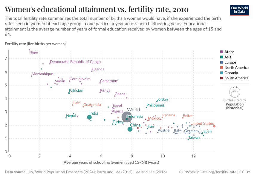
The chart below shows a fairly strong negative correlation (r =-0.8203) between the education of women in a country (average years of schooling of women in reproductive age) and the fertility rate in that country (average live births per woman). This shows that countries where women in reproductive age tend to have more education, are also countries where women tend to have fewer children.

The correlation coefficient does not necessarily tell the whole story of the relationship between two variables. For example, the relationship between fertility rates and women’s education in the chart above looks somewhat curved, and is therefore not well represented by a single number. In countries where female educational attainment is high, a given increase in female education is associated with a small decrease in fertility rates; whereas when female educational attainment is very low, the same increase is associated with a much larger decrease in observed fertility rates.

There are several other ways in which the correlation coefficient may not be fully adequate to summarise the relationship between two variables. We discuss these in a related glossary entry What’s the difference between correlation and causation?

Keywords: Causality, Correlation, Impact

Authors: N.W. Galwey & E. Ortiz-Ospina

Correlation is a relationship between two variables. For example, the weight of human individuals is correlated with their height: a tall person usually, but not always, weighs more than a short person. The correlation between two variables does not depend on the units of measurement of the variables, and it doesn’t tell us anything about the direction or source of the relationship. A causal relationship, on the other hand, is a specific type of directed cause-and-effect association between two variables. Correlation doesn’t imply causation, nor does causation imply correlation.

The chart below shows the relationship between the education of women in a country (average years of schooling of women in reproductive age) and the fertility rate in that country (average live births per woman). This shows a strong negative correlation. However, this correlation may occur because educational attainment causes changes in the number of children that women choose to have, or because having children causes changes in educational attainment. In fact, it may also be that neither variable directly influences the other, but that both are responding to some other, perhaps unobserved, variable: for example, countries where women tend to have higher educational attainment may also be countries where female labor force participation is higher, and it may be this factor that is causing differences in reproductive outcomes. To decide which explanation is more reasonable, we must have other information. (As it turns out, the available evidence suggests education does contribute to explain fertility, and you can read more about it here).

If we have information on a third variable for each observation, we can ask how strong is the correlation between the first two variables after adjusting for the third. For example, in the case of education and fertility, employment and female labor force participation rates across countries are also available, so we can find the correlation coefficient between fertility rates and educational attainment after controlling for differences in female employment across countries. This is called the partial correlation coefficient, and we can think of it as the correlation coefficient that would have been observed if all countries had the same level of female labour force participation. It takes us one step further to understand the interaction between the variables.

However, a partial correlation is still not sufficient to identify a causal relationship. First, the direction of the relationship is undetermined (is x causing y or is y causing x?). And second, there are always unobservable factors that may be unaccounted for. Correlation doesn’t imply causation.

Interestingly, it is also true that causation does not imply correlation. Indeed, an absence of correlation between two variables does not necessarily indicate that they are independent. For example, consider the height of an arrow at different moments in time after it is shot vertically from a bow. There is an exact relationship between the time and the height: if you know the time in seconds since the arrow was shot, you can tell exactly how high the arrow will be. However, time and height are uncorrelated – on average, over the whole range of time while the arrow is in the air, a later time is not associated with a greater or lesser height.

Correlations are informative. But there are many ways in which a correlation coefficient can conceal as much as it reveals – a collection of examples is presented here.

Keywords: Correlation, Linear correlation, Regression analysis, Regression coefficient

Authors: N.W. Galwey & E. Ortiz-Ospina

In statistics, a regression is an approach for modeling the relationship between two or more variables. In its simplest form, regressing two variables requires finding a line of best fit to describe the relationship between them.

To provide the intuition behind this concept, let us consider first the related concept of correlation. Correlation is a relationship between two variables. For example, the weight of human individuals is correlated with their height: a tall person usually, but not always, weighs more than a short person. The correlation between two variables does not depend on the direction of the relationship between them. However, the related statistical concept of ‘regression’ captures both the strength and direction of the relationship.

In regression analysis, the direction of the relationship between the variables comes from treating one of them as the ‘response’ variable (or the ‘dependent’ variable), and the other as the ‘explanatory’ (or ‘independent’) variable.

For example, a regression analysis can be performed to relate the education of women in a country (the explanatory variable) and the fertility rate in that country (the response variable); as show in the chart below. Loosely speaking, regressing fertility on education requires ‘finding the line of best fit’, which essentially means drawing a straight line in a way that ensures the points in the scatter plot are as close as possible to the drawn line.

The line of best fit is often used to make predictions. In this example, the line could be used as a model, where the slope of the line (the ‘regression coefficient’) tells us the change in number of children per woman that would be associated with every additional year of schooling.

Two important points are worth emphasising. First, the order and unit of measurement of the variables matters: if education is measured differently, or if it is used as the response variable, then the regression coefficient will be different. And second, the fact that the model allows making predictions doesn’t necessarily mean that those predictions are good.

Indeed, regression coefficients can be expressed in terms of correlation coefficients (here is the mathematical derivation). And since correlation does not imply causation, it is often the case that a simple regression model is not, on its own, a good instrument to make predictions.

– ‘Seeing Theory’ is a beautiful free online textbook on statistics that includes a chapter on regression analysis.

Keywords: Confidence interval, Selection bias

Authors: N.W. Galwey & E. Ortiz-Ospina

When we want to understand the relationship between variables, we typically attempt to estimate it using data from a sample. A ‘confidence interval’ is a statistical method that gives us an indication of just how accurate our sample estimate is.

For example, the correlation coefficient between weight and height, calculated from a sample of schoolchildren in a specific city, can be used as an estimate of the correlation in the whole population of schoolchildren in the country. If the school we choose to estimate this correlation is large and typical for the country, then we would expect this estimate to be close, but not exactly the same as the correlation in the whole population. Setting a ‘confidence interval’ involves using information about the dispersion of the data, in order to set lower and upper bounds on our estimate, so that we have an idea of how close the sample and population estimates are: in this example, how close the school-level estimate is to the general country-level relationship.

Confidence intervals can be constructed for any type of statistical estimate. The chart below, for example, shows the estimated average impact of organic farming, relative to conventional farming, on a number of dimensions (from this post). These estimates come from averaging impacts across studies in different settings. Here, if a dot is very close to ‘1’, then it means that organic and conventional farming tend to have on average a similar impact on that specific dimension. The ‘whiskers’ below and above the dots, are the confidence interval. These whiskers give us an idea of how accurate the estimates of the impacts are.

Consider the purple dot and whiskers under the block labelled ‘Greenhouse gas emissions’. Since the whiskers cross the horizontal line at ‘1’, it means that based on the sample of studies considered, we can’t rule out that organic and conventional farming have a similar impacts on emissions in general. (This is why on this chart, the whiskers are grayed out whenever they do not cross ‘1’).

An important caveat is that confidence intervals require making assumptions about how the sample relates to the population. In its simplest form, confidence intervals assume that a sample is a random subset of the population. In many social situations, this assumption is violated by ‘selection bias’.

Selection bias arises from the method of collecting data. For example, if you measure an outcome of interest for patients who self-select into a medical study, you will likely have a biased sample, because those who self-selected are often different from those who do not sign up for the study, and may therefore not be representative of the overall population intended to be analyzed.

In the Wikipedia entry on selection bias you find more examples and technical explanations.

Keywords: Statistical significance test, Statistical hypothesis testing, p-value.

Authors: N.W. Galwey & E. Ortiz-Ospina

We are often interested in knowing whether there is clear evidence of a particular relationship between two variables. For example, how strong is the evidence against the hypothesis that two variables are uncorrelated? We can ask this question by performing a ‘significance test’. When we perform such a test, a statistical metric called the ‘p-value’ helps us interpret the result.

When we want to understand the relationship between variables, we typically attempt to estimate these relationships using data from a sample. For example, the correlation coefficient between weight and height, calculated from a sample of schoolchildren in a specific city, can be used as an estimate of the correlation in the whole population of schoolchildren in the country. If the school from which we select the children to estimate this correlation is a large and typical school for the country, then we would expect this estimate to be close, but not exactly the same as the correlation in the whole population of chilren.

A significance test may be one-sided or two-sided, depending on whether we have a prior expectation concerning the direction of any relationship between the variables. For example, it is appropriate to perform a one-sided test of the correlation between the weight and height of schoolchildren, because we expect that if there is a true relationship between these variables it will be positive.

The probability that an estimated correlation could occur by chance if there were no real relationship (i.e. if r = 0) is indicated by the so-called ‘p-value’ from such a test. This is a probability value between 0 and 1, a small p-value is interpreted as significant evidence of a real relationship.

p-values can be obtained for any hypothesis test involving statistical estimates. For example, we could run an experiment where we test whether a particular intervention (e.g. cash transfers for the poor) has an impact on an outcome of interest (e.g. work). We would estimate the impact for a representative sample of individuals, and then we would run a statistical significance test to assess a hypothesis (e.g. how likely is it that cash transfers have no discouraging effect on work?).

A small p-value would tell us that we have strong evidence to reject the hypothesis (e.g. reject the baseline conjecture that cash transfers have no effect on work). And conversely, a large p-value would tell us that we cannot reject the hypothesis. Crucially, however, it should be kept in mind that failure to reject a hypothesis is not the same as decisively accepting it. Absence of evidence is not the same as evidence of absence.

An article in Vox explains it as follows.

Rejecting the null [hypothesis] is like the “innocent until proven guilty” principle in court cases […] In court, you start off with the assumption that the defendant is innocent. Then you start looking at the evidence: the bloody knife with his fingerprints on it, his history of violence, eyewitness accounts. As the evidence mounts, that presumption of innocence starts to look naive. At a certain point, jurors get the feeling, beyond a reasonable doubt, that the defendant is not innocent.

Interpreting p-values also requires caution for other reasons. First, how ‘small’ is a ‘small p-value’ is a non-trivial question. In most academic studies, p-values below 0.05 are considered small, but this is the subject of much debate. And second, it should be kept in mind that a very small relationship between two variables may well be statistically significant, but this does not imply that it should have any practical significance. Practical significance is context-specific.

The poverty headcount ratio is an indicator of the incidence of poverty. It is calculated by counting the number of people in a country living with incomes or consumption levels below a given poverty line, and dividing this number of poor people by the entire population in the country.

Measuring poverty through the headcount ratio provides information that is straightforward to interpret; it tells us the share of the population living with consumption (or incomes) below the poverty line.

But measuring poverty through headcount ratios fails to capture the intensity of poverty – individuals with consumption levels marginally below the poverty line are counted as being poor just as individuals with consumption levels much further below the poverty line.

The poverty gap index is an alternative way of measuring poverty that considers the intensity of deprivation.

For more information, data and analysis on poverty headcount ratios, check our entry on Global Extreme Poverty

The International Poverty Line is the threshold used measure extreme poverty. The World Bank is the main source for global information on extreme poverty today and sets the International Poverty Line. This poverty line was revised in 2022 – since then a person is considered to be in extreme poverty if he or she is living on less than 2.15 international dollars (int.-$) per day, at 2017 PPP prices.

See our Poverty page for information, data and research. For a discussion of how the International Poverty Line is set, see our article From $1.90 to $2.15 a day: the updated International Poverty Line.

Synonyms: PPP adjustments; PPP rates;

Purchasing power parity rates (PPP rates), are conversion rates used to adjust for cross-country differences in price levels. PPP rates allow translating monetary values in local currencies into ‘international dollars’ (noted int-$). International dollars are a hypothetical currency used as common unit of measure for making cross-country comparisons of monetary indicators of standards of living.

Purchasing power adjustments are necessary because making meaningful cross-country comparisons of standards of living requires ensuring that the data subject to comparison is expressed in the same ‘unit of measure’.

Choosing a common unit of measure is not straightforward when it comes to measuring standards of living through money-metric indicators such as household consumption or average national incomes, because the underlying data is typically calculated in ‘local currency units’.

One way to deal with this is to simply translate all national figures into one common currency (for instance, US dollars) using exchange rates from currency markets. But because market exchange rates do not always reflect the different price levels between countries, economists often opt for a different alternative. They create a hypothetical currency, called ‘international dollars’, and use this as a common unit of measure. The idea is that a given amount of international dollars should buy roughly the same amount – and quality – of goods and services in any country.

The exchange rates used to translate monetary values in local currencies into ‘international dollars’ (int-$) are the ‘purchasing power parity conversion rates’ (also called PPP conversion factors).

In our blog you can read more about where PPP rates come from and why they are useful

International dollars are a hypothetical currency used as common unit of measure for making cross-country comparisons of monetary indicators of standards of living.

International dollars adjust monetary indicators, such as consumption and income, to account for differences in prices between countries. The idea is that a given amount of international dollars should buy roughly the same amount – and quality – of goods and services in any country, at a given point in time.

The exchange rates used to translate monetary values in local currencies into international dollars are the ‘purchasing power parity conversion rates’ (also called PPP conversion rates).

International dollars are often expressed in ‘constant PPP prices’, in order to adjust for changes in the value of money over time (i.e. inflation).

To express monetary values in international dollars at constant prices it is necessary to make two conversions. First, it is necessary to bring monetary values to a base year (something typically done using consumer price indexes); and then it is necessary to convert the values in local currencies at the base year into international dollars using PPP rates for the same year.

For more information, check our blog post What are PPP adjustments and why do we need them?

The poverty gap index is a measure that reflects both the depth and prevalence of poverty. It is defined as the mean shortfall of the total population from the poverty line, counting the non-poor as having zero shortfall and expressed as a percentage of the poverty line. 

It is worth unpacking that definition a little. For those below the poverty line, the shortfall corresponds to the amount of money required in order to reach the poverty line. For those at or above the poverty line, the shortfall is counted as zero. The average shortfall is then calculated across the total population – both poor and non-poor – and then expressed as a share of the poverty line.

Unlike the more commonly-used metric of the headcount ratio, the poverty gap index is thus sensitive not only to whether a person’s income falls below the poverty line or not, but also by how much – i.e. to the depth of poverty they experience.

Economists use the term ‘poverty trap’ to denote a situation in which individuals are stuck in deprivation over long periods of time, and there is nothing they can do by themselves to escape such situation. The term captures a situation in which poverty today causes poverty in the future, so households that start poor, remain poor.

Insufficient nutrition, for example, can lead to a poverty trap. More precisely, if physical capacity to work increases nonlinearly with food intake at low levels (i.e. if the first calories that we consume are used by our body to survive, rather than to provide the strength required to work), it is possible that those in extreme poverty get stuck in a perverse equilibrium characterized by low incomes and low nutrition: poor nutrition then becomes both the cause and consequence of poor incomes.

Conceptually, poverty traps can also take place at a collective ‘macro’ level. For example, low-income countries may lack good growth fundamentals (e.g. technology, education and infrastructure, etc.) in order to support high saving rates leading to productivity gains that would be necessary to raise national incomes.

The concept of poverty traps is important in the context of policy, since it implies that one-off policy efforts that make it possible to ‘escape the trap’ have permanent positive effects. This is the rationale often used to argue for ‘big push’ macro policies – such as the expansion of micro-finance in low-income countries. They are meant to trigger a virtuous circle betwen more savings, more investment and economic growth.

For more information, data and analysis on poverty traps check our entry on Global Extreme Poverty

People are considered to live in ‘relative poverty’ if their living conditions are below those of a particular group of people at a particular point in time. In most cases, relative poverty is measured with respect to a poverty line that is defined relative to the median income in the corresponding country.

The idea behind measuring poverty in relative terms is that the degree of deprivation depends on the relevant reference group; hence, people are typically considered poor by this standard if they have less income and opportunities than other individuals living in the same society.

Relative poverty can be considered a metric of inequality, since it measures the distance between those in the middle and those at the bottom of the income distribution.

Relative poverty can be measured using the poverty headcount ratio and the poverty gap index. Indeed, these indicators are common in Europe.¹

Relative poverty is not the same as absolute poverty. People are considered to live in ‘absolute poverty’ if their living conditions are below a fixed minimum standard of living. Typically, absolute poverty is measured through consumption or income. So people are considered poor if their income or consumption falls below a monetary threshold that is constant across time. You can read more about this in our related glossary entry What is Absolute Poverty?.

People are considered to live in ‘absolute poverty’ if their living conditions are below a fixed minimum standard of living. Typically, absolute poverty is measured through consumption or income. So people are considered poor if their income or consumption falls below a monetary threshold that is constant across time.

Absolute poverty measures are often used by governments to monitor the evolution of living conditions at the national level. Absolute poverty lines are therefore anchored, so that it is possible to make comparisons relative to a minimum consumption or income level over time.

Absolute poverty measures are also often used to compare poverty between countries. In these cases, the poverty thresholds are held constant both across time and across countries. The International Poverty Line is the best known poverty line for measuring absolute poverty globally.

Absolute poverty is not the same as relative poverty. People are considered to live in ‘relative poverty’ if their living conditions are below those of a particular group of people at a particular point in time. In most cases, relative poverty is measured with respect to a poverty line that is defined relative to the median income in the corresponding country.

For more information, data and analysis regarding poverty check our entry on Global Extreme Poverty.

A Randomised Control Trial (RCT) is a technique used to evaluate the causal effect of an intervention, such as a medical treatment or a public policy. RCTs require administering the intervention under evaluation to a random group of individuals (the ‘treatment group’) and assessing the impact by comparing outcomes against another group of individuals who were not affected by the intervention (the ‘control group’).

This is the idea behind medical trials. Today, RCTs have become increasingly popular for research in the social sciences.

You can read more about RCTs in the broader context of policy evaluations from the Abdul Latif Jameel Poverty Action Lab.

The Gini coefficient – or Gini index – is a measure of the degree of inequality in the distribution of incomes in a population. A Gini coefficient of zero represents a distribution where incomes are perfectly equally distributed. A Gini coefficient of 1 means maximal inequality (one person has all income and all others receive no income).

The Gini coefficient was developed by Italian statistician Corrado Gini (1884-1965) and is named after him.

The following figure illustrates the definition of the Gini index: in a population in which income is perfectly equally distributed, the distribution of incomes are represented by the ‘line of equality’ – 10% of the population would earn 10% of the total income, 20% would earn 20% of the total income and so on.

The ‘Lorenz curve’ shows the income distribution in a population where income is not equally distributed – in the example below you see that the bottom 60% of the population earn 30% of the total income. The Gini coefficient captures the deviation of the Lorenz curve from the ‘line of equality’ by comparing the areas A and B:

Gini = A / (A + B)

This means a Gini coefficient of zero represents a distribution where the Lorenz curve is just the ‘Line of Equality’ and incomes are perfectly equally distributed – a value of 1 means maximal inequality (one person has all income and all others receive no income).

In case you need a simpler visual explanation of the Gini you find the right-hand side panel of the above chart only here:

Carbon dioxide (CO₂) is the most important greenhouse gas (GHG), but not the only one – methane, nitrous oxide and other gases also contribute to global warming. To capture all GHG emissions, researchers therefore express them in ‘carbon dioxide-equivalents’ (CO₂eq). This metric takes account not just CO₂ but all greenhouse gases.

To express all greenhouse gases in carbon dioxide-equivalents (CO₂eq), they are each weighted by their global warming potential (GWP) value. GWP measures the relative warming impact of one molecule or unit mass of a greenhouse gas relative to carbon dioxide over a given timescale – usually over 100 years. For example, one tonne of methane would have 28 times the warming impact of tonne of carbon dioxide over a 100-year period. GWP100 values are used to combine greenhouse gases into a single metric of emissions: carbon dioxide equivalents (CO₂eq). CO₂eq is then derived by multiplying the mass of emissions of a specific greenhouse gas by its equivalent GWP100 factor. The sum of all gases in their CO₂eq form provide a measure of total greenhouse gas emissions.

To express all greenhouse gases in carbon dioxide-equivalents (CO₂eq), they are each weighted by their global warming potential (GWP) value. GWP measures the relative warming impact of one molecule or unit mass of a greenhouse gas relative to carbon dioxide over a given timescale – usually over 100 years. For example, one tonne of methane would have 28 times the warming impact of tonne of carbon dioxide over a 100-year period. GWP100 values are used to combine greenhouse gases into a single metric of emissions called carbon dioxide equivalents (CO₂eq). CO₂eq is then derived by multiplying the mass of emissions of a specific greenhouse gas by its equivalent GWP100 factor. The sum of all gases in their CO₂eq form provide a measure of total greenhouse gas emissions.

Food miles are measured in tonne-kilometers which represents the transport of one tonne of goods by a given transport mode (road, rail, air, sea, inland waterways, pipeline etc.) over a distance of one kilometre.

‘Carbon budget’ is a concept used to define the quantity of greenhouse gases we can emit over a given period of time before average warming would exceed a given level – for example, 2°C higher than pre-industrial temperatures. It is used to address the question: how much greenhouse gases can we emit before global average warming increases by more than 2°C?

Radiative forcing measures the difference between incoming energy and the energy radiated back to space. If more energy is absorbed than radiated, the atmosphere becomes warmer.

Child mortality measures the share of newborns who die before reaching the age of five.

It expresses the probability of a child born in a specific year or period dying before reaching the age of 5 years, if subject to age-specific mortality rates of that period. This is given as the share of live births.

Infant mortality measures the share of newborns who die before reaching one year of age.

It expresses the probability of a child born in a specific year or period dying before reaching the age of one, if subject to age-specific mortality rates of that period. This is given as the share of live births.

Neonatal mortality measures the share of newborns who die before reaching 28 days of age.

It expresses the probability of a child born in a specific year or period dying before reaching 28 days of age, if subject to age-specific mortality rates of that period. This is given as the share of live births.

The maternal mortality ratio measures the number of women who die from pregnancy-related causes per 100,000 live births.

A maternal death refers to the death of a woman while pregnant or within 42 days of termination of pregnancy. Included are deaths from any cause related to or aggravated by the pregnancy but not from accidental or incidental causes.

A maternal death refers to the death of a woman while pregnant or within 42 days of termination of pregnancy. Included are deaths from any cause related to or aggravated by the pregnancy but not from accidental or incidental causes.

Children per woman is measured as the total fertility rate, which is the number of children that would be born to the average woman if she were to live to the end of her child-bearing years and give birth to children at the current age-specific fertility rates.